

What Happens When AI Listens to a Song
When you press play, you hear melody, rhythm, emotion. A machine hears something entirely different: a stream of numerical samples, thousands per second, waiting to be decoded into structured information. That gap between raw signal and musical meaning is exactly what AI music analysis bridges.
What AI Music Analysis Actually Means
At its core, analyzing music with AI means converting audio into data you can search, sort, and act on. The system takes a waveform and extracts attributes like tempo, key, mood, instrumentation, and genre without a human ever pressing a tag button. Neural networks learn patterns from thousands of labeled examples, then apply that knowledge to tracks they have never encountered before.
AI music analysis is the automated extraction of musical attributes from audio signals using machine learning models trained on labeled datasets.
This process goes well beyond simple beat detection. Modern music analysis AI operates on multiple levels of abstraction simultaneously, identifying low-level statistical features like spectral centroid and energy, mid-level perceptual qualities like pitch and rhythm, and high-level semantic concepts like genre and emotional tone.
Why Understanding the Process Matters
Streaming platforms now host catalogs growing by thousands of tracks every day. Manual tagging at that scale is unrealistic. AI-driven analysis powers the recommendation engines, playlist generators, and search tools that connect listeners with music they actually want to hear. Producers use these systems for instant feedback on their mixes. Researchers leverage them to study musical patterns across entire genres and decades.
Understanding how AI analyzes music also reveals its blind spots. Every model carries assumptions baked into its training data, its architecture, and its feature extraction choices. Knowing the mechanics helps you interpret results critically rather than treating AI output as ground truth.
This article walks through the full technical pipeline, from the moment sound enters the system to the structured metadata that comes out the other end. You will see exactly what happens at each stage and why specific engineering choices shape what the machine can and cannot hear.
The Full Pipeline from Sound Wave to Structured Data
Every song analyzer, whether it powers a streaming recommendation engine or a standalone music analyzer app, follows the same fundamental sequence. Sound enters as vibrating air, and structured metadata comes out the other side. The magic lies in what happens between those two endpoints.
Here is the complete pipeline that AI systems use to analyze music:
- Analog-to-digital conversion - a microphone or file input captures air pressure changes as discrete numerical samples
- Pre-processing - the digital signal is segmented into short overlapping frames and windowed to reduce spectral artifacts
- Time-frequency transformation - each frame is converted from a waveform into a frequency representation (spectrogram)
- Feature extraction - musically meaningful descriptors are computed from the spectral data
- Model inference - trained neural networks interpret the features and produce predictions
- Post-processing - raw predictions are smoothed, thresholded, and formatted into usable output
From Waveform to Time-Frequency Representation
The journey begins with digitization. A standard audio file stores amplitude values sampled at a fixed rate, typically 44,100 Hz for CD-quality audio or 22,050 Hz for many analysis systems. That means the system captures over 44,000 snapshots of air pressure every second. These raw samples are just numbers on a timeline and reveal almost nothing about musical content directly.
To make sense of this data, the system slices the waveform into short overlapping frames, usually 20 to 25 milliseconds long, with a 10-millisecond hop between them. Each frame is multiplied by a window function (commonly a Hamming window) that tapers the edges to zero, preventing artificial frequency artifacts at frame boundaries.
A Fast Fourier Transform (FFT) then converts each windowed frame from the time domain into the frequency domain, revealing which frequencies carry energy at that moment. Stack these frequency snapshots side by side across time, and you get a spectrogram: a visual map showing frequency on one axis, time on the other, and energy as intensity.
The format of your input file matters here. Lossy compression formats like MP3 and M4A discard frequency information deemed inaudible to human listeners. A validation study published in JMIR Biomedical Engineering found that compression effects on extracted features are format-specific and bitrate-dependent, with MFCCs showing less stability than basic voice features across compression methods. For critical analysis, uncompressed WAV or lossless FLAC preserves the full spectral information a model needs.
Feature Extraction and What Each Feature Reveals
Raw spectrograms contain far more data than a model needs. Feature extraction distills this information into compact, musically relevant descriptors. When you analyze music computationally, three feature families do most of the heavy lifting:
- MFCCs (Mel-Frequency Cepstral Coefficients) - These compress the spectral envelope into roughly 13 coefficients per frame by applying a perceptually weighted mel filterbank followed by a logarithmic compression and a Discrete Cosine Transform. The result captures timbral texture: the "color" of a sound that lets you distinguish a piano from a guitar playing the same note.
- Chroma features - These map all frequency energy onto the 12 pitch classes (C, C#, D, etc.), collapsing octave information. Chroma is ideal for tracking harmony and chord progressions regardless of which octave instruments are playing in.
- Spectral centroid - This single value represents the "center of mass" of the frequency spectrum for each frame. A high spectral centroid indicates bright, treble-heavy sound; a low value suggests darker, bass-dominated timbre.
Other commonly extracted descriptors include spectral rolloff (the frequency below which a set percentage of energy falls), zero-crossing rate (useful for distinguishing pitched from percussive sounds), and tempo-related features like onset strength. Together, these features give the model a multi-dimensional fingerprint of the audio at every time step.
Model Inference and Output Post-Processing
Features feed into trained neural networks that have learned associations between these numerical patterns and musical labels. The model outputs raw predictions, often as probability distributions. A genre classifier might return 0.72 for "jazz," 0.18 for "soul," and 0.10 for "R&B" for a single track.
These raw outputs rarely go straight to the user. Post-processing refines them: temporal smoothing averages predictions across neighboring frames to eliminate flickering results, confidence thresholding discards low-probability labels, and aggregation collapses frame-level predictions into track-level or segment-level summaries. A beat tracker, for example, might detect onset candidates at every frame but then apply a dynamic programming step to select the most rhythmically consistent beat grid.
The entire pipeline, from sample to structured output, typically runs in seconds for a single track. Scale that across millions of songs, and you understand why this architecture underpins every major music analyzer in production today. Each stage introduces design choices that shape accuracy, and the most consequential of those choices happens at the spectrogram level, where the system decides how to "see" the frequency content of sound.
How AI Sees Music Through Spectrograms
That "seeing" is more literal than you might expect. Any AI that can listen to audio does so by first converting sound into an image-like representation. Neural networks, particularly convolutional architectures borrowed from computer vision, need spatial structure to detect patterns. Spectrograms provide exactly that: a two-dimensional map where the x-axis is time, the y-axis is frequency, and pixel intensity represents energy. Feed a spectrogram into a CNN and the network treats it much like a photograph, scanning for local patterns that correspond to musical events.
How Spectrograms Turn Sound into Images
Imagine slicing a song into thousands of tiny windows, each a few milliseconds long, and asking "which frequencies are active right now?" Stack those frequency snapshots left to right, and you get a spectrogram. Low frequencies sit at the bottom, high frequencies at the top, and brighter regions indicate louder energy. A sustained bass note appears as a persistent bright band near the bottom. A cymbal crash lights up the upper frequencies in a brief vertical streak.
This visual approach is also biologically plausible. Our own cochlea performs a similar frequency decomposition along the basilar membrane, converting pressure waves into a spatial frequency map before signals reach the brain. Spectrograms mirror that process digitally, which partly explains why they work so well for classification tasks grounded in human perception.
Not all spectrograms are equal, though. The choice of frequency scaling and resolution directly shapes what the model can detect. Three types dominate audio AI dynamics in music research, and each reveals different musical properties.
Mel-Spectrograms vs Constant-Q Transform vs STFT
The standard STFT uses linear frequency spacing: every bin covers the same number of Hertz. This gives you raw, even resolution across the entire spectrum, which is useful for detecting sharp transients and percussive onsets. The trade-off is size. A typical STFT produces 1,025 frequency bins, most of which represent high-frequency ranges where musical content is sparse.
Mel-spectrograms solve this by applying a perceptual filter bank that compresses high frequencies and expands low frequencies, approximating how the human ear perceives pitch. Below 1,000 Hz the scale is roughly linear; above that it becomes logarithmic. The result? A compact representation, often just 128 mel bins instead of 1,025 STFT bins, that still captures the spectral detail listeners actually care about. Research consistently shows mel-spectrograms outperform other spectral representations for classification tasks using deep CNNs. They are the default choice when you are unsure what AI can listen to audio for and need a general-purpose input.
The Constant-Q Transform takes a different approach. Its frequency bins are spaced logarithmically and aligned directly with musical note intervals, providing equal resolution per octave. You get excellent pitch discrimination in the low and mid ranges, making CQT ideal for harmony analysis, chord detection, and pitch tracking. The cost is higher computational complexity and less software availability compared to mel-spectrograms.
| Type | Frequency Resolution | Best Use Case | Trade-offs |
|---|---|---|---|
| STFT | Linear (equal Hz per bin) | Transient detection, percussive onset analysis | Large output size; wastes bins on sparse high-frequency regions |
| Mel-Spectrogram | Perceptual (mel scale) | Timbre, mood, genre classification | Irreversible compression; frequency detail lost at high ranges |
| Constant-Q Transform | Logarithmic (octave-aligned) | Pitch tracking, harmony, chord recognition | Computationally heavy; no perfect reconstruction; fewer library implementations |
In practice, what ai can listen to audio for depends heavily on which spectrogram feeds the model. A mood classifier benefits from the perceptual weighting of mel-spectrograms. A chord transcription system gains accuracy from CQT's note-aligned bins. And a drum onset detector might prefer the raw temporal precision of a high-resolution STFT.
These spectral images are just the input layer, though. What the network does with them, the architecture it uses to scan for patterns and build higher-level understanding, determines whether the system merely detects frequencies or truly interprets musical structure.
Neural Network Architectures Behind Music AI
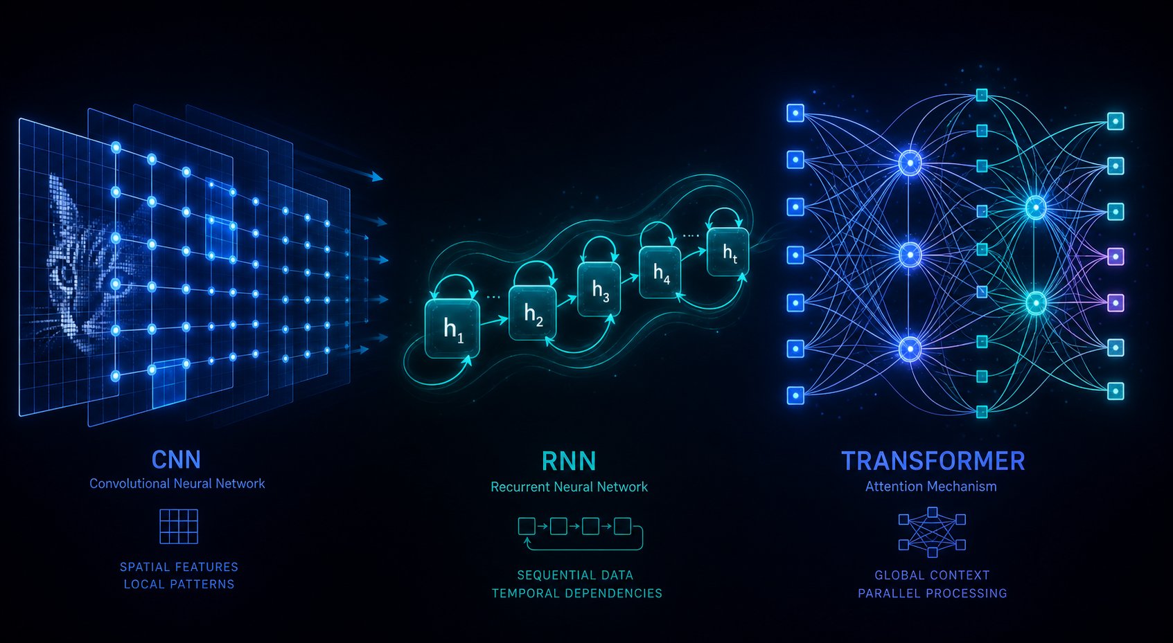
The architecture scanning those spectrograms is where musical understanding actually takes shape. Three families of neural networks dominate how AI analyzes music, and each one "listens" in a fundamentally different way. Think of it like three musicians in a studio: one focuses on tone color, another follows the melody line through time, and the third steps back to grasp the entire song structure at once.
CNNs and Pattern Recognition in Spectrograms
Convolutional Neural Networks were originally designed to classify photographs, but they adapt remarkably well to spectrograms. A CNN slides small filters (typically 3x3 grids) across the time-frequency image, detecting local patterns: the harmonic stack of a trumpet, the broadband burst of a snare hit, or the energy distribution that distinguishes a distorted guitar from a clean one.
Early layers learn basic spectral shapes. Deeper layers combine those shapes into higher-level concepts like "piano chord" or "breathy vocal." This hierarchical feature extraction is why CNNs excel at timbre recognition, instrument detection, and short-term rhythmic features. Research on music classification architectures shows that even relatively simple CNN designs like the Fully Convolutional Network (FCN) or VGG-ish models achieve strong tagging performance by stacking convolutional layers with batch normalization and max-pooling to progressively widen the receptive field.
The limitation? Standard CNNs process fixed-size patches. They see local texture clearly but struggle to connect a chorus at the 30-second mark to its reprise two minutes later. A CNN-based song analyzer captures what a sound is, but not necessarily how it relates to what came before or after.
RNNs for Tracking Musical Sequences Over Time
Music unfolds sequentially. A chord progression only makes sense in order. A melody builds tension through the notes that precede the resolution. Recurrent Neural Networks, particularly Long Short-Term Memory (LSTM) variants, are built for exactly this kind of sequential reasoning.
An LSTM processes spectrogram frames one at a time, maintaining a hidden state that carries information forward. Each new frame updates that internal memory, allowing the network to track temporal dependencies: how a melody contour rises and falls, when a chord change occurs, and how rhythmic patterns evolve across measures.
In practice, though, standalone RNNs face a challenge. Feeding raw mel-spectrogram frames (128-dimensional vectors at each time step) directly into an LSTM forces the recurrent layer to simultaneously learn spectral features and temporal structure. A comparative study on music genre classification found that a standalone LSTM achieved only 68% accuracy on mel-spectrogram input, actually underperforming some classical machine learning models. The raw spectral data proved too complex for the recurrent layer to process without prior feature extraction.
This weakness becomes a strength when you pair the RNN with a CNN front end. The convolutional layers first compress the spectrogram into a sequence of abstract feature vectors, then the LSTM models how those features evolve. This sequential CRNN (Convolutional Recurrent Neural Network) design achieved 84% accuracy in the same study, a 13-point improvement over the best classical approach and 16 points above the standalone RNN. The CNN "cleans up" spectral information so the LSTM can focus entirely on temporal patterns.
Transformers and Long-Range Musical Structure
LSTMs process sequences step by step, which means information from early in a song must survive through every intermediate step to influence predictions later. For long pieces, that chain becomes fragile. Transformers solve this with self-attention: every position in the sequence can directly attend to every other position, regardless of distance.
Imagine a song analysis AI trying to recognize that the guitar riff at 3:20 is a variation of the one at 0:15. An LSTM must carry that memory through three minutes of intervening data. A transformer can directly compare those two moments in a single attention computation. This makes transformers particularly effective for detecting repetition, identifying song sections (verse, chorus, bridge), and understanding overall form.
The Music Transformer introduced by Google Magenta demonstrated that relative attention, which encodes the distance between events rather than their absolute position, captures structural patterns like repeated motifs, call-and-response phrases, and scale patterns more effectively than vanilla self-attention. This relative position awareness aligns naturally with how music works: a perfect fifth interval matters regardless of which octave it appears in.
Modern music tagging transformers typically pair a CNN front end with a transformer back end. The CNN extracts local acoustic features from short spectrogram chunks, and the transformer summarizes those features across the full duration using self-attention. This hybrid approach also provides interpretability: attention heatmaps reveal which parts of the audio contribute most to each predicted tag, giving users visibility into the model's reasoning.
The table below summarizes how these three architectures compare for song analysis AI tasks:
| Architecture | Strengths | Typical Tasks | Limitations |
|---|---|---|---|
| CNN | Local pattern detection; efficient on fixed-size inputs; strong timbre discrimination | Instrument classification, mood tagging, onset detection | No native temporal modeling; misses long-range dependencies |
| RNN (LSTM) | Sequential memory; tracks temporal evolution; models transitions | Chord progression tracking, melody transcription, beat tracking | Struggles with raw high-dimensional input; slow to train on long sequences; information decay over distance |
| Transformer | Direct long-range attention; parallelizable training; interpretable attention maps | Song structure segmentation, repetition detection, full-track tagging | High memory cost for long sequences; requires large training data; less inductive bias for local patterns |
In production systems, you rarely encounter a pure architecture. The most effective AI song analyzer designs combine components: a CNN front end for spectral feature extraction feeding into a transformer or LSTM back end for temporal summarization. This modular approach lets each component do what it does best, spectral pattern recognition in one stage and sequential reasoning in the next.
Architecture determines what the model can learn, but what it actually learns depends on something else entirely: the data it trains on. The composition of training datasets, the labels humans assign, and the cultural assumptions baked into those labels shape the boundaries of what any song analyzer AI can reliably detect.
Training Data and How It Shapes What AI Hears
A model's architecture defines what it can learn. Training data defines what it does learn. Even the most powerful transformer is only as perceptive as the examples it was trained on, and in music AI, those examples carry deep assumptions about what music is, how it should be categorized, and whose listening perspective counts as ground truth.
How Labeled Datasets Teach AI to Hear
Supervised learning, the backbone of most music classification systems, requires labeled examples. Human annotators listen to tracks and assign tags: genre, mood, instrumentation, structural boundaries, key, tempo. The model then learns statistical associations between audio features and those human-provided labels. When it encounters a new track, it predicts labels based on patterns it absorbed during training.
Standard Music Information Retrieval (MIR) datasets illustrate both the power and limitations of this approach. DEAM provides 1,802 music excerpts with continuous arousal-valence emotion annotations. CAL500 contains 502 songs tagged with multiple emotion labels. EMOPIA covers multi-modal pop piano data for emotion recognition. These corpora have driven years of research, but their relatively small scale, often just hundreds or thousands of tracks, constrains model generalization.
Several factors determine whether a trained model produces reliable results or confidently wrong ones:
- Dataset size - Larger datasets expose the model to more variation, reducing overfitting to narrow patterns
- Genre diversity - A model trained only on pop and rock will misinterpret jazz voicings or classical ornamentation
- Annotator agreement - When labelers disagree, the model learns from noise rather than consistent patterns
- Audio quality consistency - Mixing pristine studio recordings with lo-fi field recordings introduces confounding variables
- Label granularity - Coarse labels like "happy" versus "sad" teach less nuance than dimensional scales like valence and arousal
The labeling challenge runs deeper than logistics. Genre is famously subjective: is a track "indie rock" or "alternative"? Mood perception varies from person to person. A study on music emotion annotation found that even trained human experts with similar cultural backgrounds achieved a Fleiss' Kappa of only 0.561 when categorizing classical piano pieces into emotion quadrants, meaning substantial natural disagreement exists in what should count as the "correct" label. Any AI music reviewer inherits this ambiguity directly from its training signal.
Cultural Bias and the Limits of Training Data
Here is where training data creates real blind spots. A study from MBZUAI presented at NAACL surveyed over one million hours of music across existing training datasets and found that nearly 94% represented Western genres. Only 0.3% came from Africa, 0.4% from the Middle East, and 0.9% from South Asia. In total, just 5.7% of training data represented non-Western music.
The consequences are predictable. Models trained on this distribution rely on Western tonal conventions, 12-tone equal temperament, and standard time signatures even when processing music that follows entirely different rules. A system built on these datasets may misclassify microtonal intervals in Turkish Makam as "out of tune," interpret complex polyrhythmic cycles in West African drumming as irregular timing, or fail to recognize instruments like the sitar, oud, or kora that simply were not in the training distribution.
Attempts to fix this through fine-tuning show promise but also reveal how deep the problem runs. The same MBZUAI researchers applied parameter-efficient adapters to retrain models on Hindustani classical and Turkish Makam styles. The fine-tuned systems improved on those specific genres, but their performance on Western styles began to degrade. The models started "forgetting" what they had previously learned, suggesting that surface-level patches cannot substitute for genuinely diverse training data from the outset.
For anyone relying on an AI music rater or automated tagging system, this bias is not abstract. It means the confidence scores and genre labels you see are most trustworthy for well-represented styles, typically Western pop, rock, electronic, and classical, and least reliable for traditions outside that narrow slice. An honest ai music review of any track should acknowledge where the model's training gives it authority and where it is essentially guessing.
These dataset limitations set a ceiling on accuracy, but they are not the only factor. Even within well-represented genres, AI systems face tasks where pattern matching hits a wall: interpreting irony, parsing emotional nuance, or making sense of deliberately unconventional production.

Where AI Excels and Where It Still Struggles
Pattern matching hits a wall exactly where human interpretation begins. When you analyze the song purely on measurable attributes, tempo, key, spectral patterns, AI systems perform remarkably well. But music carries meaning that lives outside the waveform: cultural context, irony, deliberate rule-breaking. That divide between signal processing and musical understanding defines the current state of the field.
Where AI Outperforms Human Listeners
For tasks that reduce to consistent, quantifiable patterns, machines are fast and reliable. A 2025 benchmark comparing four leading analysis platforms showed near-unanimous agreement on BPM detection, key identification, and primary genre classification across well-produced pop, hip-hop, and folk tracks. All four systems correctly identified the key and tempo of Kendrick Lamar's "Not Like Us" within one BPM of each other. Beat tracking, repetitive structure detection, and instrument identification in cleanly mixed recordings are similarly strong. An AI song rater can process thousands of tracks per hour at this level of accuracy, something no human team could match.
Tasks That Still Challenge AI Models
Accuracy drops sharply once you move beyond well-structured, well-produced music. The same benchmark revealed significant disagreements when analyzing more complex productions. "Die With a Smile" by Bruno Mars and Lady Gaga produced BPM estimates ranging from 105 to 158 across different analyzers, and key predictions spanned three different values. When systems attempt to analyze song ai-style at the level of mood or cultural nuance, divergence grows further.
Electronic music with rigid quantization and clear spectral separation is AI's comfort zone. Free jazz, avant-garde composition, or heavily layered lo-fi recordings push models into territory their training never adequately covered. And tasks requiring interpretive judgment, distinguishing parody from sincerity, understanding why a dissonance is intentional, or recognizing that a genre violation is the artistic point, remain beyond reach.
| AI Strengths (High Accuracy) | AI Limitations (Lower Reliability) |
|---|---|
| Tempo and BPM detection in steady-tempo tracks | Emotional nuance and cultural context |
| Key identification in tonal music | Genre classification for experimental or boundary-crossing music |
| Beat tracking and onset detection | Distinguishing irony, parody, or intentional rule-breaking |
| Instrument classification in clean mixes | Analyzing heavily layered or lo-fi recordings |
| Repetitive pattern and structure recognition | Understanding musical intention and artistic context |
| Primary genre classification for well-represented styles | Non-Western rhythmic cycles and microtonal systems |
The honest takeaway: AI excels at answering "what is happening sonically?" and struggles with "what does it mean?" For producers, curators, and researchers, this distinction matters. Use automated analysis confidently for measurable attributes, but treat mood tags, genre labels for unconventional music, and emotional assessments as suggestions rather than verdicts. The system knows what it heard. It does not always know what it means.
These capabilities and constraints are not just academic. They shape how real products behave, from the recommendation engine that surfaces your next favorite track to the source separation tool that isolates a vocal stem for remixing.

Real-World Applications Beyond Tagging and Cataloging
Recommendation engines, stem splitters, educational platforms, therapy tools: the same analytical pipeline powering genre tags and BPM readouts feeds into products that reshape how people create, learn, and experience music every day. The applications span far beyond metadata generation, touching nearly every corner of the music industry.
- Recommendation and playlist generation - clustering songs by sonic similarity to build taste profiles at scale
- Source separation - isolating vocals, drums, bass, and other stems from finished mixes
- Music education - delivering instant feedback on pitch accuracy, timing, and technique
- Music therapy - adapting playlists based on detected emotional content and physiological response
- Copyright detection - fingerprinting audio and matching it against registered catalogs
- Live performance analysis - monitoring intonation, dynamics, and ensemble balance in real time
Recommendation Engines and Playlist Generation
When a streaming platform suggests your next track, it is not simply matching genre labels. Modern recommendation systems combine multiple approaches. Collaborative filtering predicts preferences based on user similarity, essentially recreating the "friend with great taste" at algorithmic scale. Content-based filtering analyzes the audio itself, extracting embeddings that represent how a track sounds in a form that can be compared across millions of songs. Context-aware systems factor in time of day, activity, and listening environment.
Each approach has trade-offs. Collaborative filtering creates filter bubbles, reinforcing what you already like rather than expanding your horizons. It also suffers from the cold-start problem: new tracks with no listening history cannot be recommended until users interact with them. Content-based analysis sidesteps both issues by evaluating audio directly, meaning a brand-new upload can surface in recommendations immediately based on sonic similarity alone. Most production systems now blend all three approaches, using AI mix analysis of audio features alongside behavioral signals to balance familiarity with discovery.
Source Separation for Creators and Learners
Source separation takes the analytical pipeline in a different direction entirely. Instead of describing what is in the mix, the model reconstructs individual components. You upload a finished stereo file, and AI estimates what the vocals, drums, bass, and remaining instruments probably sound like in isolation.
This works because the same pattern recognition that identifies "there is a drum kit in this track" can be extended to predict exactly which portions of the mixed signal belong to that drum kit. Modern separation models like Hybrid Transformer Demucs process both the waveform and spectrogram simultaneously, using transformer layers to reason about musical context across time. The waveform branch preserves transient detail and timing; the spectrogram branch recognizes harmonic and frequency patterns.
The results are not perfect reconstructions of the original studio session. They are informed estimates. But for practical workflows, those estimates are remarkably useful. MakeBestMusic's Audio Separator puts this technology in the hands of musicians, students, remixers, and creators who want to inspect individual parts of a track without needing to install Python, configure GPU drivers, or navigate command-line tools. Upload a song, choose your separation mode, and download isolated stems you can study, practice with, or remix. This kind of audio AI dynamics music analyzer makes it possible to pull apart a professional mix and hear exactly how the bass interacts with the kick drum, or how the vocal sits relative to the instrumentation.
For producers studying arrangement techniques, the ability to solo individual stems from reference tracks transforms passive listening into active analysis. For students learning an instrument, isolated parts reveal fingerings, phrasing, and dynamics that get buried in the full mix.
Music Education, Therapy, and Copyright Detection
Music feedback AI is reshaping how students practice. Pitch detection algorithms compare a student's played notes against a reference in real time, highlighting intonation errors, timing drift, and rhythmic inconsistencies the moment they happen. Instead of waiting for a weekly lesson, a learner gets instant corrective signals that accelerate skill development. Some platforms even track progress over weeks, showing measurable improvement in accuracy and consistency.
Music therapy applies the emotional analysis side of the pipeline. Therapists use AI-curated playlists that adapt based on detected mood characteristics, matching arousal and valence levels to therapeutic goals. A session targeting relaxation pulls low-energy, consonant tracks; one designed to energize selects higher-tempo, brighter material. The system does not replace clinical judgment, but it handles the catalog search problem, surfacing appropriate music from thousands of options in seconds.
Copyright detection relies on audio fingerprinting, a specialized form of analysis that generates compact, robust identifiers from short audio segments. These fingerprints remain stable across format changes, compression, speed shifts, and even partial recordings captured from a live environment. Platforms match uploaded content against registered databases of millions of tracks, flagging potential infringements within seconds of upload. The same core technology powers broadcast monitoring, ensuring rights holders know when and where their music plays.
Live performance analysis brings the pipeline into real-time territory, monitoring intonation, balance, and dynamics as musicians play. Orchestras use these tools during rehearsal to identify sections where individual players drift from ensemble tuning. Solo performers get post-session reports showing exactly where their timing loosened or their pitch wandered.
Each of these applications depends on the same foundational pipeline: waveform in, structured understanding out. The difference lies in what happens after inference. A recommendation engine uses embeddings for similarity search. A separation tool uses learned patterns to reconstruct sources. An education platform uses pitch tracking for corrective feedback. The analytical core is shared; the product layer determines who benefits and how.
All of this raises a practical question: if you want to explore how AI interprets music firsthand, where do you actually start?
Getting Started with AI Music Analysis Tools
Reading about pipelines, spectrograms, and neural architectures builds conceptual understanding. But the fastest way to internalize how AI interprets music is to feed it a track you know well and examine what comes back. The gap between what you hear and what the system reports teaches more than any technical paper.
Fortunately, you do not need a machine learning degree or a GPU cluster to start experimenting. Music analysis tools span a wide range of accessibility, from zero-setup browser apps to full Python libraries for building custom pipelines. Here is a practical map of your options.
Browser-Based Tools for Instant Analysis
The lowest-friction entry point is a browser-based analyzer. Upload a file or paste a link, and you get back key, BPM, energy profile, and sometimes mood or genre tags within seconds. These tools run inference on remote servers, so your local hardware does not matter.
Several free ai music analyzer options let you test basic extraction immediately:
- Key and BPM detectors - Services like Tunebat and Song Key Finder return tonal center and tempo from any uploaded track. Useful for DJs preparing sets or producers matching samples to a project key.
- Full-spectrum taggers - Platforms like Cyanite's web app analyze mood, genre, instrumentation, energy, and more across dozens of categories. These give you a feel for what commercial-grade tagging produces.
- Waveform and spectral viewers - Tools that display real-time spectrograms alongside playback help you visually connect what you hear to what the model sees. Try uploading a track with a distinctive instrument entrance and watch the spectrogram light up at that moment.
These browser tools are excellent for building intuition quickly. Run the same track through two or three different analyzers and compare results. You will notice they sometimes disagree on key, mood, or genre, which mirrors the accuracy limitations discussed earlier. That disagreement is itself informative: it reveals where the analysis is confident versus where interpretation varies.
Source Separation as a Learning Tool
If tagging tells you what is in a mix, separation shows you how it fits together. Pulling a track apart into individual stems, vocals, drums, bass, and other instruments, is one of the most revealing ways to understand both the music and the AI processing it.
MakeBestMusic's Audio Separator is a strong starting point for non-technical users who want to separate and inspect parts of a track without writing code or configuring local environments. Upload a song, select your separation mode, and download isolated stems ready for study or creative use. The interface removes the technical barriers that typically sit between a curious listener and hands-on analysis.
Other separation tools worth exploring include:
- MakeBestMusic Audio Separator - Browser-based, no install required. Separates vocals, drums, bass, and accompaniment. Ideal for musicians, students, and remixers who want quick access to individual stems.
- Moises - Web and mobile app with vocal, drum, bass, guitar, and piano separation. Includes pitch and tempo adjustment for practice use.
- Ultimate Vocal Remover 5 - Free, open-source desktop application with multiple model options. More complex to set up, but offers fine-grained control over separation algorithms.
- Lalal.ai - Web and desktop app using a proprietary neural network. Offers a wide range of instrument stems including strings, wind, and individual guitar types.
Try separating a track you have mixed or produced yourself. Compare the AI's estimated stems against your original multitracks. Where the model nails it, you are seeing the strength of its learned patterns. Where it struggles, bleeding instruments or missing harmonics, you are seeing the limits of current separation technology in real time.
Open-Source Options for Developers
If you want to build custom analysis pipelines or understand the mechanics at the code level, open-source libraries give you full control. Python dominates this space, with mature packages covering every stage of the pipeline discussed in this article.
Librosa is the standard starting point. Install it with a single command (pip install librosa) and you immediately have access to spectrogram generation, MFCC extraction, chroma features, beat tracking, onset detection, and tempo estimation. Its documentation includes introductory tutorials that walk you from loading an audio file to extracting meaningful features in a few lines of code.
Beyond librosa, the ecosystem includes:
- Essentia - A comprehensive C++/Python library from the Music Technology Group at Universitat Pompeu Fabra, covering audio analysis, descriptors, and pre-trained models for classification tasks.
- Madmom - Focused on beat tracking, downbeat detection, and rhythm analysis with state-of-the-art recurrent neural network models.
- Demucs - Meta's open-source separation model that you can run locally for high-quality stem extraction with full control over parameters.
For developers, the real value is not just running these tools but chaining them together. Extract features with librosa, feed them into a classifier you train on your own labeled data, and post-process the output into whatever format your application needs. You are rebuilding the same pipeline that powers commercial music analysis tools, just with full visibility into every decision point.
Whatever entry point matches your skill level, the key is hands-on experimentation. Run the same track through multiple tools. Compare a browser tagger's genre prediction against a separation tool's isolated stems against your own ears. Notice where systems agree, where they diverge, and where your musical knowledge catches things the AI misses entirely. That comparison builds a practical understanding of both the power and the boundaries of how AI interprets music, one track at a time.
